Introduction to Sinusoidal Signal Processing with Scilab

This article discusses basic signal-processing tasks that can be performed using a free and open source alternative to MATLAB.

Scilab vs. MATLAB

I’ve done quite a bit of work with MATLAB over the years, and it is undoubtedly a powerful tool that can simplify and accelerate a wide variety of engineering tasks. However, developing software of this quality is by no means inexpensive, and I wouldn’t be surprised to learn that the cost of a standard MATLAB license doesn’t fit within the budgetary constraints of numerous entrepreneurs, consultants, startups, and small engineering firms. It turns out, though, that there is an alternative to MATLAB that is completely free called Scilab.

In my experience with Scilab, it is very capable and reasonably user-friendly. Another advantage is that the Scilab interface is similar to the MATLAB interface, so if you have experience with MATLAB (maybe from your days as a student or an employee of a large company), Scilab should feel somewhat familiar.

Working with Digitized Sinusoids

In the world of signal processing, sinusoids are everywhere. This is as true in the digital realm as it is in the analog realm, and consequently it is important to thoroughly understand the nature of a digitized sinusoid.

Both analog and digital sine waves have amplitude, frequency, and phase. For this article, we don’t need to concern ourselves with phase, and amplitude doesn’t really change when you move from analog to digital; frequency, on the other hand, requires some attention. In the analog domain, frequency specifies the number of cycles with respect to time. Units of time are the same always and everywhere—e.g., 100 Hz (= 100 cycles per second) means the same thing in every engineering project. In the digital domain, frequency loses its reference to an unchanging unit of time. Instead, we have individual amplitude values that must be interpreted according to the sample rate. This can lead to confusion for two reasons: 1) many different sample rates are used, and 2) sample-rate information is not contained within the series of amplitude values.

Sine Generation in Scilab

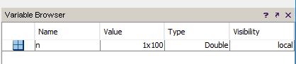
Let’s explore this issue through an example. We’re going to use Scilab to create one cycle of a sine wave that has 100 samples per cycle. This is the first command:

n = 0:99;

We just created an array that begins at 0 and ends at 99. You can look in the “Variable Browser” to confirm that n is a one-dimensional array with a length of 100.



The array n is the digital equivalent of t (i.e., time) in the typical sin(ωt) expression that we use in the analog domain. Next, I’ll enter the following two commands:

y = sin(n);
plot(y)

This is the result:



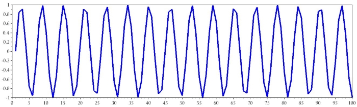
It looks terrible, I know, and it’s clearly wrong—we wanted one cycle composed of 100 samples. Let’s think about why this happened:

1. Sine is simply a function that operates on an argument.
2. The sine function does not generate unique values for every argument. Rather, the values repeat when the argument changes by 2π: sin(0) = sin(2π) = sin(4π) = sin(6π)....
3. Thus, one cycle of sine values corresponds to a 2π range of argument values.
4. This means that to generate one cycle of sine values, we need to modify the argument array so that it extends from 0 to 2π.

The command y = sin(n) doesn’t produce the desired waveform because the argument given to the sine function is an array that extends from 0 to 99. The solution is to divide n by the desired number of samples per cycle, which in this case is 100, and also multiply it by 2π:

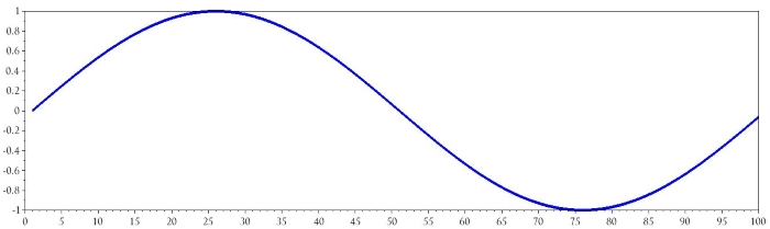
y = sin(2*%pi*n/100);

You can readily confirm that this will work: if n is zero, the entire argument is zero; if n is 100, the argument is (2π × 100/100) = 2π; and all the numbers in between are scaled accordingly. Thus, we have reduced the argument range to 2π, and we are still producing 100 samples. (Note: I realize that in this case n does not extend to 100, but if it did, we would want the value 100 to be the first sample in the second cycle. In other words, the first cycle is covered by the 100 values from 0 to 99, the second cycle would be covered by the 100 values from 100 to 199, and so forth.) Here is the result:

plot(y)

Refining the Plot

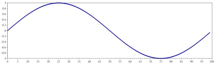
There’s still something not quite right about the plot. We know that sin(0) = 0, but in the plot, the waveform has a value of 0 for a horizontal-axis value of 1. In other words, the waveform is shifted one sample to the right. This occurs because we didn’t specify a list of horizontal-axis values that correspond to the vertical-axis values contained in the array y. If we tell Scilab plot(y), it uses default values for the horizontal axis, and apparently these default values start at one.

The command y = sin(2*%pi*n/100) generates y values that correspond to the numbers in the array n. If we want the plot to maintain this relationship between y and n, we can use the following command:

plot(n, y)

Incorporating Frequency and Sample Rate

When we’re working with real sinusoidal signals, we generally think in terms of signal frequency (in the analog domain) and sampling frequency (in the digital domain). Thus, we need to integrate these parameters into the purely mathematical ideas presented thus far.
Fortunately, this is not difficult. We saw above that the argument for the sine function needs to include a factor of (2π/samples per cycle). We can calculate samples per cycle for real-world signals as follows:

    

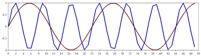
Let’s say we have a system that digitizes a 6 kHz audio signal and a separate 2 kHz audio signal. The sampling frequency is 44.1 kHz, and the ADC fills a 50-sample buffer. The following sequence of Scilab commands can be used to generate values that resemble the data produced by the actual system.

SignalFrequency_1 = 6e3;
SignalFrequency_2 = 2e3;
SamplingFrequency = 44.1e3;
n = 0:49;
Signal_1 = sin(2*%pi*n / (SamplingFrequency/SignalFrequency_1));
Signal_2 = sin(2*%pi*n / (SamplingFrequency/SignalFrequency_2));
plot(n, Signal_1)
plot(n, Signal_2)

Conclusion

This article provided a brief introduction to the characteristics of digitized sinusoids and the techniques used to create these sinusoids in Scilab. I plan to write additional articles on Scilab-based signal processing and analysis; if there’s a specific topic that you think would be interesting, feel free to mention it in the comments.