Basics of Digital Down-Conversion in DSP

This article discusses digital down-conversion which is a digital-signal-processing technique widely used in digital radio receivers.

Digital down-conversion is a digital-signal-processing technique that is widely used in digital radio receivers. This article will review the basics of a digital down-converter (DDC). We’ll first look at the advantages of using a DDC rather than its analog counterpart. Then, we’ll discuss an example and explore the basic operation of a DDC.

To understand the advantages of using a DDC, let’s first review a traditional dual-down-conversion receiver and examine its drawbacks. The basic dual-down-conversion receiver is shown in Figure 1. As you can see, there are several analog blocks before the signal is digitized by the analog-to-digital converters (ADC).

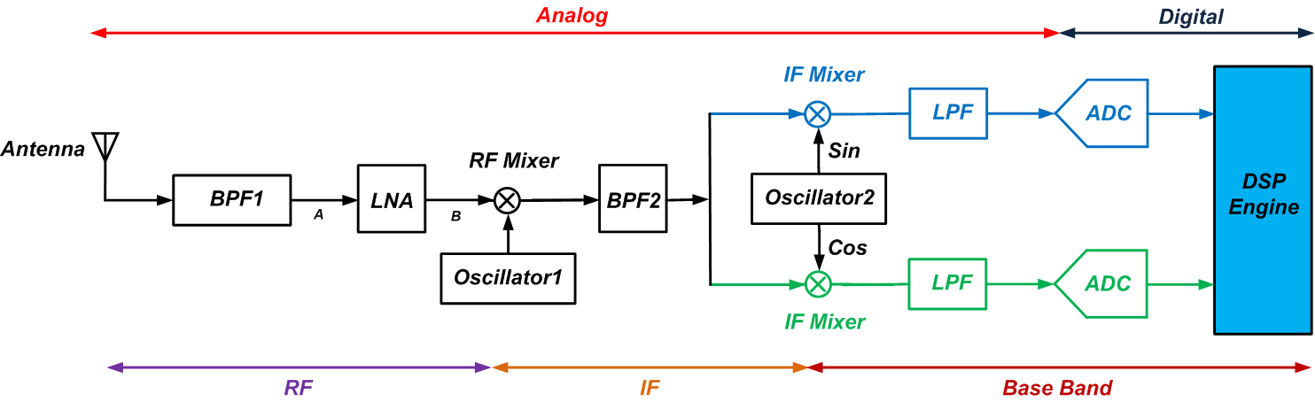
Figure 1. Click to enlarge.

The following section reviews the basic functionality of each of the blocks used in the above receiver. If you’re familiar with the basics of RF engineering, you can go through the next section to refresh your knowledge; otherwise, you may want to begin by reading some pages from AAC’s RF textbook.

The Basic Dual-Down-Conversion Receiver

In the receiver of Figure 1, the first bandpass filter, BPF1, performs image rejection for the first mixer, labeled “RF Mixer” in the figure. It also partially suppresses the interferers picked up by the antenna. This relaxes the linearity requirements of the low-noise amplifier (LNA).

The output of the bandpass filter is amplified by the LNA. This amplification makes the noise that will be contributed by the following stages relatively small in comparison to the desired signal. In this way, the receiver becomes less sensitive to the noise of the stages after the LNA.

Then, the amplified signal at node B is down-converted to the intermediate frequency, [Math Processing Error]

, by the RF mixer.
Now that the desired signal has been down-converted to a lower frequency, we can more easily build a relatively high-Q filter, BPF2, and partially perform the channel selection. Note that, thanks to the dual-down-conversion structure of the receiver, the intermediate frequency of the first mixer, [Math Processing Error]

, can be relatively high. This relaxes the requirements of BPF1.
Next, the signal goes through a quadrature mixer driven by Oscillator 2 (see Figure 1). The frequency of Oscillator 2 is equal to [Math Processing Error]
, so that the center frequency of the desired band will be translated to DC. This means that we won’t need an image rejection filter for the IF mixers.

Next we perform channel selection by means of the baseband low-pass filters (LPFs), and finally, the ADCs will digitize the desired signal and the result will be further processed by the digital signal processor (DSP). The DSP engine will perform operations such as equalization, demodulation, and channel decoding.

Drawbacks to the Traditional Radio Receiver and the Solution

We can consider three main limitations of the dual-down-conversion receiver shown in Figure 1:

1. The two baseband paths must be highly matched. The IF mixer, LPF, and ADC in the blue path must be matched with the corresponding components in the green path.
2. The analog filters introduce phase distortion.
3. The ADCs inject a DC term that cannot be easily removed from the desired information. Note that the IF mixers of Figure 1 translate the center frequency of the desired channel to DC, where the ADC can inject an error term. This ADC offset can be produced by the offset of its building blocks such as amplifiers and comparators. The offset term leads to a non-zero digital code even when a zero signal is applied to the ADC. This can be very important in systems that convey information at very low frequencies.

We could remedy these imperfections in the DSP portion of the receiver; however, a better solution would be putting the A/D converter before the quadrature mixers in the receiver chain. This is shown in Figure 2.

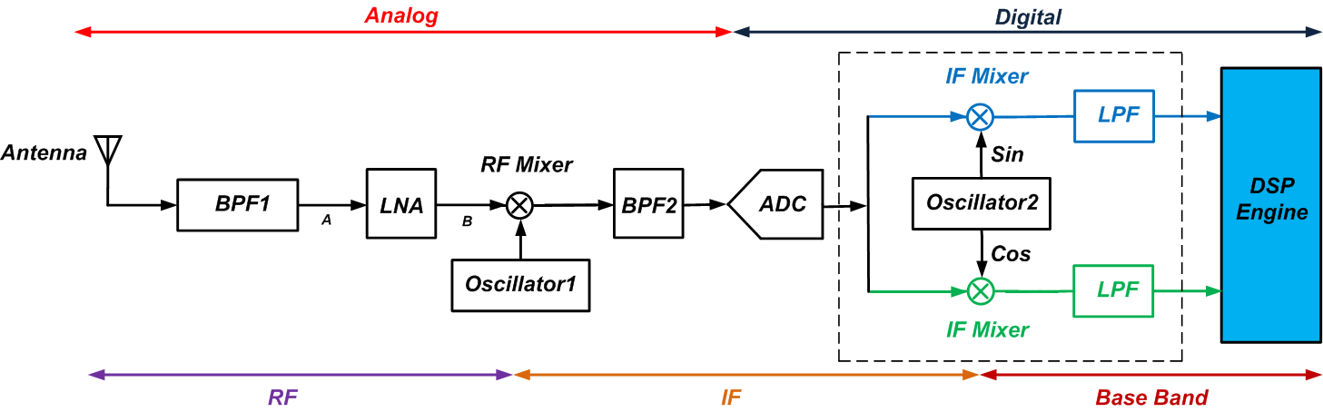
Figure 2. Click to enlarge.

As you can see, now the A/D conversion takes place at the IF rather than at baseband. This means that the ADC will have to operate at a higher sample rate. As shown in the figure, the blocks after the ADC are all operating in the digital domain. For example, the outputs of Oscillator 2 in Figure 2 are actually the digital values corresponding to the sine and cosine signals. To implement Oscillator 2, we generally use a direct digital synthesizer (DDS). The second down-conversion is performed using two digital multipliers, and the LPFs are digital filters.

As mentioned above, with the structure of Figure 2, the ADC will have to operate at a higher sample rate. This could be considered a disadvantage, but the DDC approach also offers significant benefits:

1. Now, the IF mixers and the LPFs are digital circuits. Hence, imbalance-related distortions, which arise from the mismatch between analog components, have been eliminated.
2. Unlike in the analog domain, we can easily design linear-phase digital filters.
3. The DC term injected by the ADC can easily be removed by a digital filter before the signal goes through the IF mixers (see chapter 12 of Digital Front-End in Wireless Communications and Broadcasting for an example).

Note that, while Figure 2 has the quadrature mixers and LPFs outside of the receiver’s DSP engine, we could certainly implement these blocks within the system’s DSP platform. Also, after the baseband LPF, we can reduce the sample rate significantly without losing the desired information (see my article on multirate DSP and its application in A/D conversion for more information). Thus, we can redraw the circuitry inside the dashed box of Figure 2 as shown in Figure 3. This block is called a digital down-converter, or DDC.

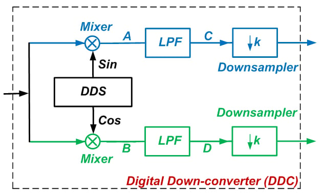
Figure 3

Digital Down-Conversion

Let’s assume that after analog-to-digital conversion the spectrum of the desired signal is as shown in Figure 4.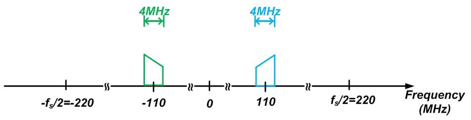

Figure 4

The desired signal is centered at 110 MHz, and it has a bandwidth of 4 MHz (the diagram shows both the positive and the negative frequencies). Also, we assume that the ADC is producing samples at a rate of 440 MSPS (mega samples per second). How will the DDC process this input?
The DDS employed by the DDC will generate 110 MHz sine and cosine signals. Each of these sine and cosine functions will lead to impulses at [Math Processing Error]

MHz. Since multiplication in the time domain corresponds to convolution in the frequency domain, we will get the spectrum shown in Figure 5 for nodes A and B in Figure 3.

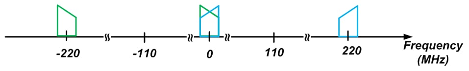
Figure 5

As you can see, a frequency shift of [Math Processing Error]

MHz has translated the blue spectrum of Figure 4 to both 220 MHz and DC. Similarly, the green spectrum is shifted to both DC and -220 MHz. We are able to use one plot for nodes A and B because these two nodes have the same amplitude characteristics, and Figure 5 conveys only the amplitude spectra. The phase spectrum of node A will be different from the phase spectrum of node B.

In Figure 5, note that the signal sidebands overlap around DC after downconversion. Considering this overlap, can we recover the desired information using only the part of the spectrum that is centered around DC? Yes we can; we are using quadrature mixing, which generates two identical amplitude spectra but also two non-identical phase spectra, and the phase spectra of the overlapping region allow us to recover the original information. Since this overlap is not a problem, the frequency components above 2 MHz don’t provide any necessary information, and consequently we can put an LPF after the digital mixer to keep only the frequency components below 2 MHz. This low-pass filtering, depicted as a single-stage filter in Figure 3, is generally implemented as a two-stage filter, as shown in Figure 6.

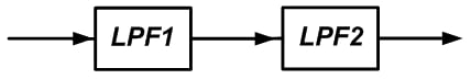
Figure 6

The first stage, LPF1, can be designed to eliminate the high-frequency components centered at 220 MHz. To this end, we need an LPF with a passband that extends to about 2 MHz and a stopband that begins at about 218 MHz. This filtering operation is sometimes referred to as filtering the image signal created by the DDS.

The second stage, LPF2, eliminates any unwanted frequency components between 2 MHz and 218 MHz. After LPF2, the signal contains no frequency components beyond the intended information bandwidth (i.e., 2 MHz), but we are still using 440 MSPS to represent this signal. Hence, we can apply the downsampling concept to reduce the sample rate.

A more efficient implementation would be to break LPF2 into a cascade of stages and perform part of the overall downsampling after each of these stages. Again, for more details about FPGA implementation of a DDC, please read Chapter 12 of the book I mentioned above.

Conclusion

In this article, we examined the benefits of using a DDC. We saw that a DDC can improve the performance of the basic dual-down-conversion receiver: It can eliminate imbalance-related distortion created by an analog IF mixer and it avoids phase distortion from analog filters. After the DDC, the sample rate is significantly reduced and we can have a more efficient implementation of the DSP routines that further process the data. 


To see a complete list of my articles, please visit this page.