DNL and INL Specifications of a DAC: Interpreting INL Shape

This article will examine some properties of the DNL and INL specifications.

In a previous article, we introduced the DNL and INL specifications. Moreover, we examined the relation between these two linearity metrics. This article will try to develop an intuitive understanding of some properties of the DNL and INL specs.

Before reading on, we strongly suggest you quickly review the previous article, What Are the DNL and INL Specifications of a DAC? Non-Linearity in Digital-to-Analog Converters.

Review of the INL Specification

The ideal transfer function of a three-bit unipolar DAC is shown in Figure 1.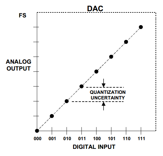

Figure 1. Image courtesy of Analog Devices.

In a real-world implementation, the DAC output voltage levels may deviate from the above ideal characteristic (see the exaggerated example shown in Figure 2).

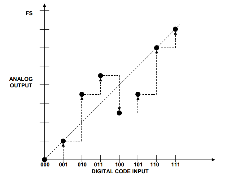
Figure 2

The INL for each output level is defined as the deviation of the actual input–output characteristic from the ideal transfer curve. For example, the INL of the output for code 100 is -1.5 LSb in Figure 2 (the ideal output should be 4 LSb but the actual output is 2.5 LSb).

Implications of an INL Less Than ±0.5 LSb

In this section, we’ll examine the implications of an input–output characteristic that exhibits an INL less than +0.5 LSb and greater than -0.5 LSb. (Note that many books would say that this DAC has an INL less than ±0.5 LSb; from a strict mathematical perspective, this statement is not accurate, but we’ll use it because it’s common and more convenient.) Let’s first examine the monotonicity of this DAC. The output of a monotonic DAC is non-decreasing for an increase in the input digital code.
The question is: Can we have a DAC with INL less than ±0.5 LSb that exhibits a non-monotonic transfer characteristic? In other words, is it possible to have a decrease in the output for an increase in the digital code while INL is less than ±0.5 LSb? If the DAC linearity errors affect two successive output levels in the opposite direction, we may have a decreasing transfer curve.

For example, in Figure 3, the output level for the code 011 is increased while the output level for 100 is decreased. The non-ideal output levels for the 011 and 100 inputs are represented by the blue and green points in the figure.

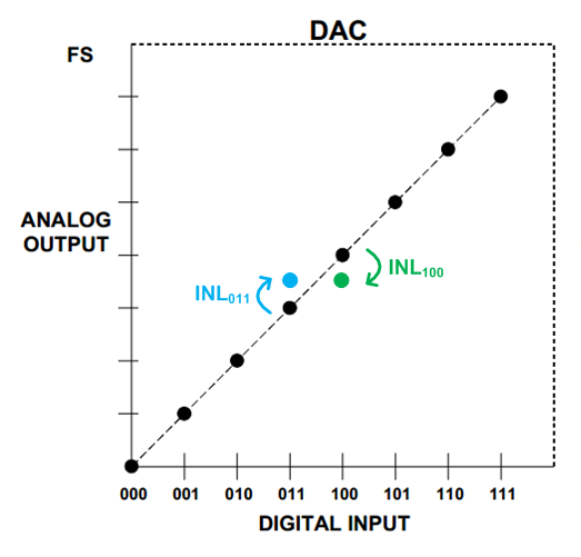
Figure 3

Obviously, a large linearity error can move the green point below the blue one. However, the DAC INL is less than ±0.5 LSb. Hence, in the worst-case scenario, we have INL011=+0.5 LSb and INL100=-0.5 LSb. The ideal difference between successive output levels is one LSb. Therefore, we cannot have a decreasing characteristic (the DAC is monotonic) if the INL is less than ±0.5 LSb.

Calculating the DNL of This DAC

What about the DNL of a DAC that has an INL less than ±0.5 LSb? Can we find an upper limit for the DNL of this DAC?

The DNL is the deviation of an output step from the ideal analog LSb value. The worst-case scenario will be as shown in Figure 4, where the linearity error reduces one output level but increases the next one.

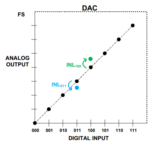
Figure 4

The maximum deviation corresponds to the case where INL₀₁₁=-0.5 LSb and INL₁₀₀=+0.5 LSb. The ideal difference between successive output levels is one LSb. Therefore, the largest possible step at the DAC output will be 2 LSb, which gives a DNL of 1 LSb. Hence, if the INL is less than ±0.5 LSb, the DNL is no more than ±1 LSb.

To summarize our discussion so far, if the INL of a DAC is less than ±0.5 LSb, the input–output characteristic is monotonic and the DNL is no more than ±1 LSb.

It’s worthwhile to mention that monotonicity does not necessarily mean that the INL is less than ±0.5 LSb. For example, the input–output characteristic of a Kelvin divider (Figure 5 below) is inherently monotonic. If we increase the input digital code, the output analog voltage will either increase or (in the worst-case scenario) retain its value; it will not decrease.

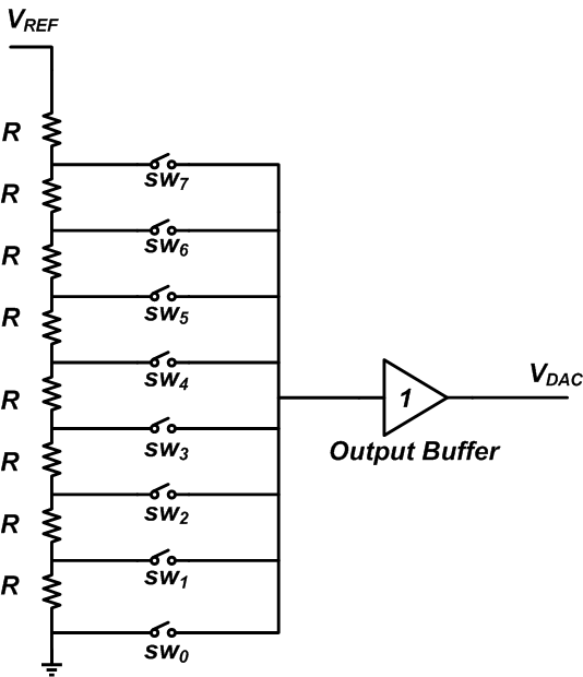
Figure 5

Assume that we have mismatch between the resistors and that the actual values are as shown in Figure 6.

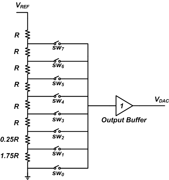
Figure 6

In this case, both the DNL and the INL for the digital code 001 (when sw1 is turned on) will be 0.75 LSb. As you can see, we have a monotonic DAC but the INL is greater than 0.5 LSb. Moreover, this example shows that even with a DNL less than ±1 LSb and a monotonic input–output characteristic, there’s no guarantee that the INL is less than ±0.5 LSb.

Interpreting the Shape of a Nonlinear Transfer Characteristic

As discussed before, the INL of a DAC is a number that gives the maximum deviation of the actual input–output characteristic from the ideal transfer curve. However, this single number cannot actually give us all the information about the DAC linearity performance.

For example, we can have two DACs with identical maximum INL that have completely different frequency domain performance.

The rest of this article will examine the effect of the INL shape on the frequency content of the DAC output. We don’t intend to give a mathematical proof; rather, we’ll focus on developing an intuitive understanding of the effect of the INL shape.

A Bow-Shaped INL

Assume that the input–output characteristic of a nonlinear four-bit DAC is as shown by the green line in Figure 7. We’ll refer to this type of INL performance as a bow-shaped INL.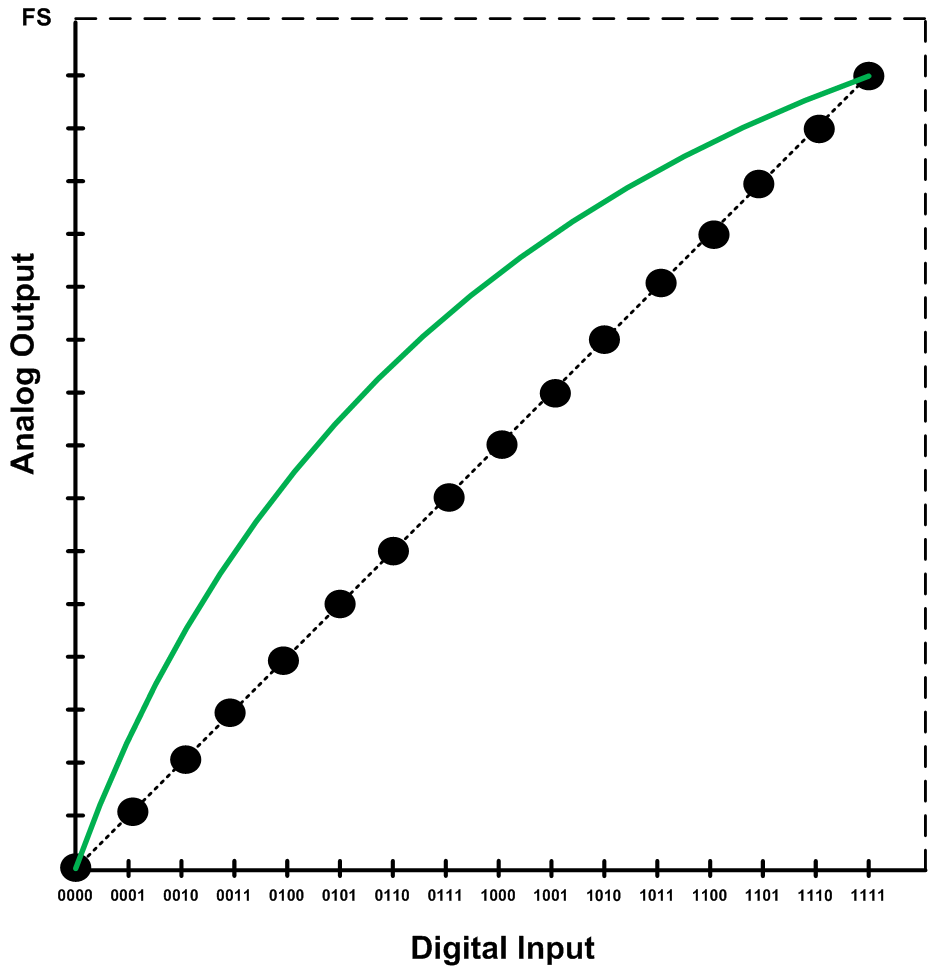

Figure 7

We know that a nonlinear DAC produces harmonic components. Let’s see what would be the dominant harmonic component of a DAC with a bow-shaped INL. To this end, we digitize a sinusoid with four bits and apply one period of this quantized sinusoid to the input–output characteristic of Figure 7. We assume that the frequency of the sinusoid is 1 kHz and that the samples are taken at 10 kHz. Figure 8 allows us to find the digital code sequence that represents this sinusoid.

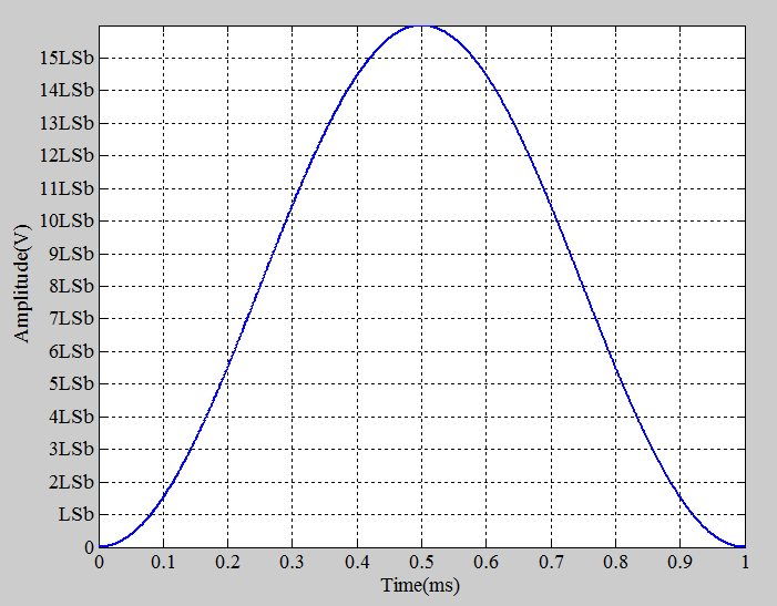
Figure 8

In this figure, the x-axis grid represents the sampling time. The y-axis grid allows us to find the digitized value of each sample. For example, the sample taken at 0.1 ms can be approximated by 1 LSb (which corresponds to the digital code 0001). The digital code sequence that should be applied to the DAC to produce one period of the sinusoid is 0000, 0001, 0101, 1010, 1110, 1111, 1110, 1010, 0101, 0001.

If the DAC were ideal, it would produce the voltage levels corresponding to the ideal characteristic (the dashed line in Figure 7). The red bars in Figure 9 show these ideal values at the sampling instants.

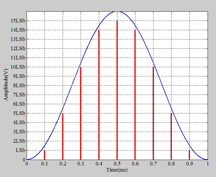
Figure 9

Since the DAC is not ideal, we’ll have some error added to each output level. For the hypothetical nonlinear characteristic of Figure 7, the error voltages correspond to the green bars in Figure 10.

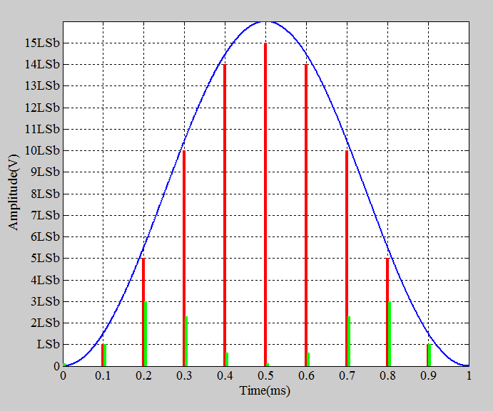
Figure 10

The actual values that the DAC produces are the sum of the value represented by a red bar and the value represented by the corresponding green bar. We know that the red bars represent a 1 kHz sinusoid. What about the green bars? Can we consider them as samples of a sinusoid of a particular frequency? As shown by the cyan curve in Figure 11, the error terms resemble the samples of a sinusoid at 2 kHz (the second harmonic of the input sinusoid). Therefore, a bow-shaped INL leads to a “dominant” second harmonic at the DAC output.

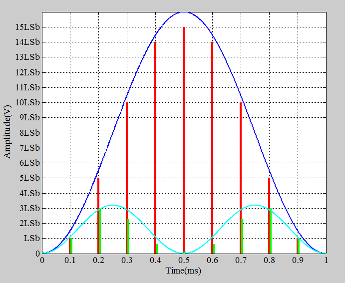
Figure 11

A Symmetric S-Shaped INL

An S-shaped INL for a four-bit DAC is shown in Figure 12.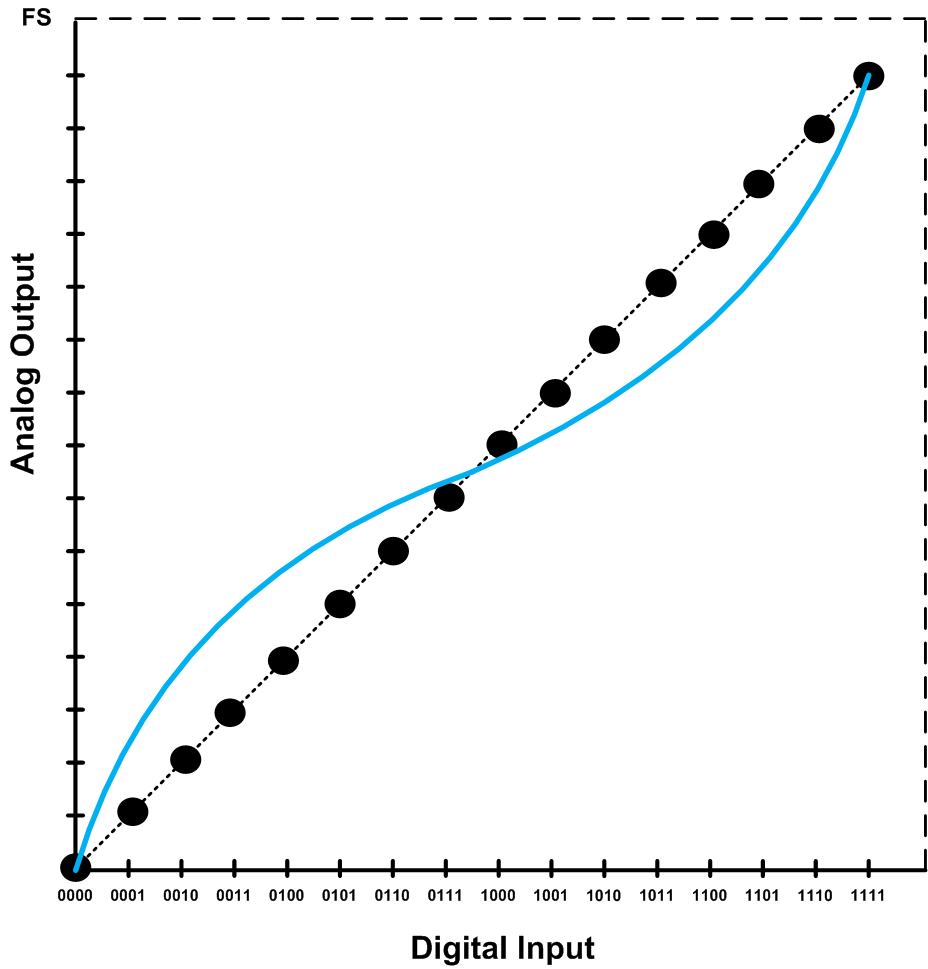

Figure 12

Again, we apply the digital code sequence representing a 1 kHz sinusoid (sampled at 10 kHz) to examine the error terms. The error terms are shown as the green bars in Figure 13.

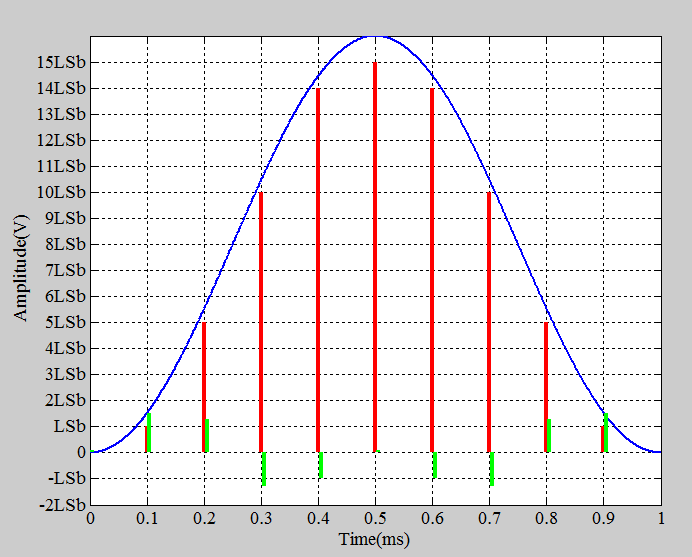
Figure 13

Note that the error terms look like samples of a function that has half-wave symmetry. A periodic function f(t) is said to have half-wave symmetry when shifting the function by half a cycle and then inverting it gives the original function f(t). Mathematically stated, f(t) has half-wave symmetry if the following is satisfied:

f(t-T/2)=-f(t)

where T denotes the period of the function. For example, the function shown in Figure 14 has half-wave symmetry (we have assumed that it’s periodic with a period of T).

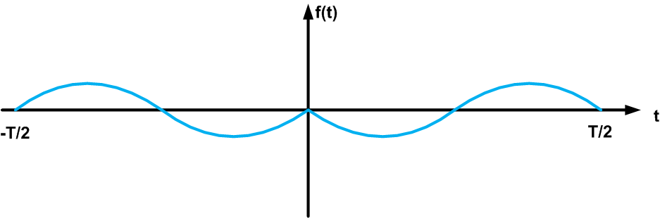
Figure 14

The error terms shown in Figure 13 are actually some samples taken from a function similar to f(t) in Figure 14. If the DAC had a higher resolution, we could have more samples and it would be easier to see the resemblance between the error samples and f(t) in Figure 14.

When a function has half-wave symmetry, it only has odd frequency components. This means that the dominant frequency component created by an S-shaped INL is the third harmonic.

To summarize, although the INL conveys information about the linearity of a DAC, this single number cannot give us all the information about the DAC’s linearity performance. We can have two DACs with identical maximum INL that have completely different frequency domain performance. If a DAC has a bow-shaped INL, the second harmonic is dominant; however, with an S-shaped INL, we expect the third harmonic to be the dominant one.

Summary

• If the INL of a DAC is less than ±0.5 LSb, the input–output characteristic is monotonic and the DNL is no more than ±1 LSb.
• With a DNL less than ±1 LSb and a monotonic input–output characteristic, there’s no guarantee that the INL is less than ±0.5 LSb.
• If a DAC has a bow-shaped INL, the second harmonic is dominant; however, with an S-shaped INL, we expect the third harmonic to be the dominant one.

To see a complete list of my articles, please visit this page.