2D Convolution in Image Processing

This article provides insight into two-dimensional convolution and zero-padding with respect to digital image processing.

In my previous article “Better Insight into DSP: Learning about Convolution”, I discussed convolution and its two important applications in signal processing field. There, the signals were presumably considered to be one-dimensional in the spatial domain. However, the process of convolution can be carried-on on multi-dimensional signals too.

In this article, we'll try to better understand the process and consequences of two-dimensional convolution, used extensively in the field of image processing.

The Definition of 2D Convolution

Convolution involving one-dimensional signals is referred to as 1D convolution or just convolution. Otherwise, if the convolution is performed between two signals spanning along two mutually perpendicular dimensions (i.e., if signals are two-dimensional in nature), then it will be referred to as 2D convolution. This concept can be extended to involve multi-dimensional signals due to which we can have multi-dimensional convolution.

In the digital domain, convolution is performed by multiplying and accumulating the instantaneous values of the overlapping samples corresponding to two input signals, one of which is flipped. This definition of 1D convolution is applicable even for 2D convolution except that, in the latter case, one of the inputs is flipped twice.

This kind of operation is extensively used in the field of digital image processing wherein the 2D matrix representing the image will be convolved with a comparatively smaller matrix called 2D kernel.

An Example of 2D Convolution

Let's try to compute the pixel value of the output image resulting from the convolution of 5×5 sized image matrix x with the kernel h of size 3×3, shown below in Figure 1.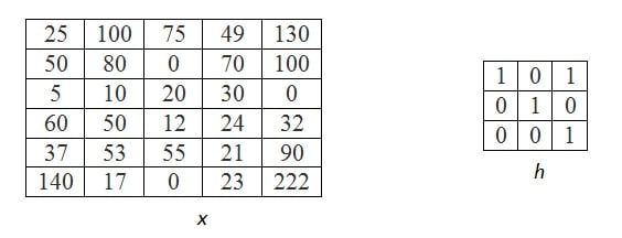

Figure 1: Input matrices, where x represents the original image and h represents the kernel. Image created by Sneha H.L.

To accomplish this, the step-by-step procedure to be followed is outlined below.

Step 1: Matrix inversion

This step involves flipping of the kernel along, say, rows followed by a flip along its columns, as shown in Figure 2.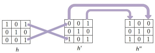

Figure 2: Pictorial representation of matrix inversion. Image created by Sneha H.L.

As a result, every (i,j)th element of the original kernel becomes the (j,i)th element in the new matrix.

Step 2: Slide the kernel over the image and perform MAC operation at each instant

Overlap the inverted kernel over the image, advancing pixel-by-pixel.

For each case, compute the product of the mutually overlapping pixels and calculate their sum. The result will be the value of the output pixel at that particular location. For this example, non-overlapping pixels will be assumed to have a value of ‘0’. We'll discuss this in more detail in the next section on “Zero Padding”.

In the present example, we'll start sliding the kernel column-wise first and then advance along the rows.

Pixels Row by Row
First, let's span the first row completely and then advance to the second, and so on and so forth.
During this process, the first overlap between the kernel and the image pixels would result when the pixel at the bottom-right of the kernel falls on the first-pixel value at the top-left of the image matrix. Both of these pixel values are highlighted and shown in dark red color in Figure 3a. So, the first pixel value of the output image will be 25 × 1 = 25.

Next, let us advance the kernel along the same row by a single pixel. At this stage, two values of the kernel matrix (0, 1 – shown in dark red font) overlap with two pixels of the image (25 and 100 depicted in dark red font) as shown in Figure 3b. So, the resulting output pixel value will be 25 × 0 + 100 × 1 = 100.

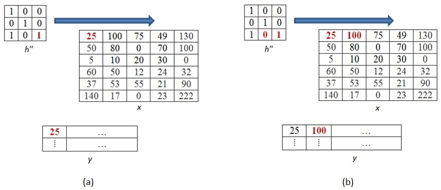
Figure 3a, 3b. Convolution results obtained for the output pixels at location (1,1) and (1,2). Image created by Sneha H.L.

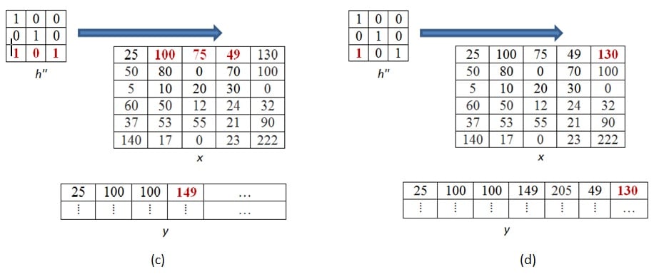
Figure 3c, 3d: Convolution results obtained for the output pixels at location (1,4) and (1,7). Image created by Sneha H.L.

Advancing similarly, all the pixel values of the first row in the output image can be computed. Two such examples corresponding to fourth and seventh output pixels of the output matrix are shown in the figures 3c and 3d, respectively.

If we further slide the kernel along the same row, none of the pixels in the kernel overlap with those in the image. This indicates that we are done along the present row.

Move Down Vertically, Advance Horizontally
The next step would be to advance vertically down by a single pixel before restarting to move horizontally. The first overlap which would then occur is as shown in Figure 4a and by performing the MAC operation over them; we get the result as 25 × 0 + 50 × 1 = 50.

Following this, we can slide the kernel in horizontal direction till there are no more values which overlap between the kernel and the image matrices. One such case corresponding to the sixth pixel value of the output matrix (= 49 × 0 + 130 × 1 + 70 × 1 + 100 × 0 = 200) is shown in Figure 4b.

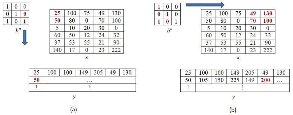
Figure 4a, 4b. Convolution results obtained for the output pixels at location (2,1) and (2,6). Image created by Sneha H.L.

This process of moving one step down followed by horizontal scanning has to be continued until the last row of the image matrix. Three random examples concerned with the pixel outputs at the locations (4,3), (6,5) and (8,6) are shown in Figures 5a-c.

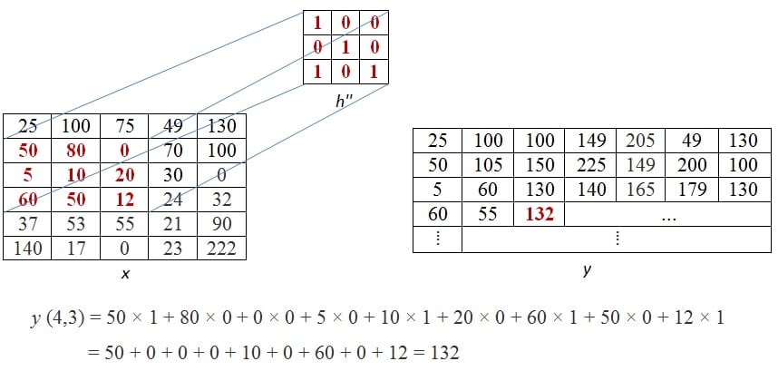
Figure 5a. Convolution results obtained for the output pixels at (4,3). Image created by Sneha H.L.

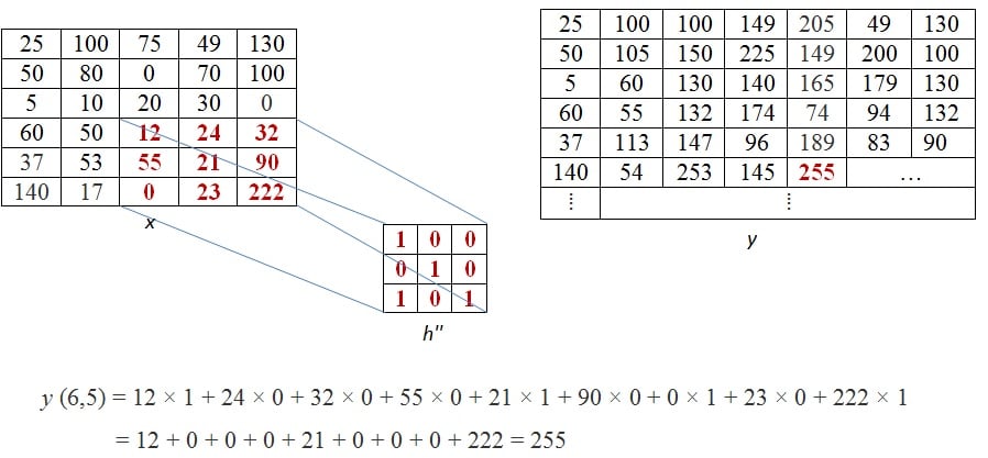
Figure 5b. Convolution results obtained for the output pixels at (6,5). Image created by Sneha H.L.

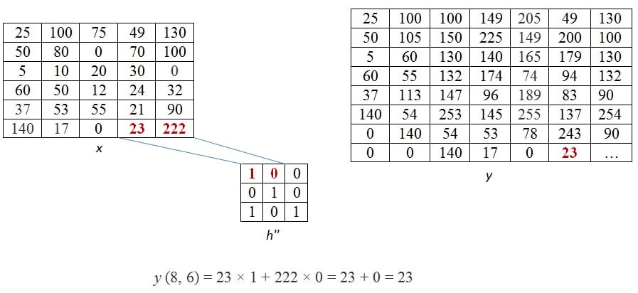
Figure 5c. Convolution results obtained for the output pixels at (8,6). Image created by Sneha H.L.

Step 

Hence the resultant output matrix will be: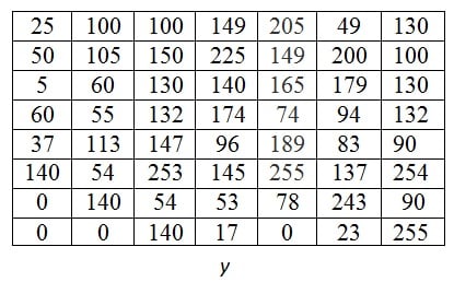

Figure 6. ​Our example's resulting output matrix. Image created by Sneha H.L.

Zero Padding

The mathematical formulation of 2-D convolution is given by

y[i,j]=∑m=−∞∞∑n=−∞∞h[m,n]⋅x[i−m,j−n]

where, x represents the input image matrix to be convolved with the kernel matrix h to result in a new matrix y, representing the output image. Here, the indices i and j are concerned with the image matrices while those of m and n deal with that of the kernel. If the size of the kernel involved in convolution is 3 × 3, then the indices m and n range from -1 to 1. For this case, an expansion of the presented formula results in

y[i,j]=∑m=−∞∞h[m,−1]⋅x[i−m,j+1]+h[m,0]⋅x[i−m,j−0]+h[m,1]⋅x[i−m,j−1]

y[i,j]=h[−1,−1]⋅x[i+1,j+1]+h[−1,0]⋅x[i+1,j]+h[−1,1]⋅x[i+1,j−1]+h[0,−1]⋅x[i,j+1]+h[0,0]⋅x[i,j]+h[0,1]⋅x[i,j−1]+h[1,−1]⋅x[i−1,j+1]+h[1,0]⋅x[i−1,j]+h[1,1]⋅x[i−1,j−1]

This indicates that to obtain every output pixel, there has to be 9 multiplications to be performed whose factors are the overlapping pixel elements of the image and the kernel. However while we computed the value for our first output pixel, we performed only a single multiplication (Figure 3a replicated as Figure 7a). What does this mean? Does it imply an inconsistency with the equation form of 2-D convolution?

No, not really. Because, the result obtained by the summation of nine product terms can be equal to the product of a single term if the collective effect of the other eight product terms equalizes to zero. One such way is the case in which each product of the other eight terms evaluate themselves to be zero. In the context of our example, this means, all the product terms corresponding to the non-overlapping (between image and the kernel) pixels must become zero in order to make the results of formula-computation equal to that of graphical-computation.

From our elementary knowledge of mathematics, we know that if at least one of the factors involved in multiplication is zero, then the resulting product is also zero. By this analogy, we can state that, in our example, we need to have a zero-valued image-pixel corresponding to each non-overlapping pixels of the kernel matrix. Pictorial representation of this would be the one as shown in Figure 7b. One important thing to be noticed here is, such an addition of zeros to the image do not alter the image in any sense except its size.

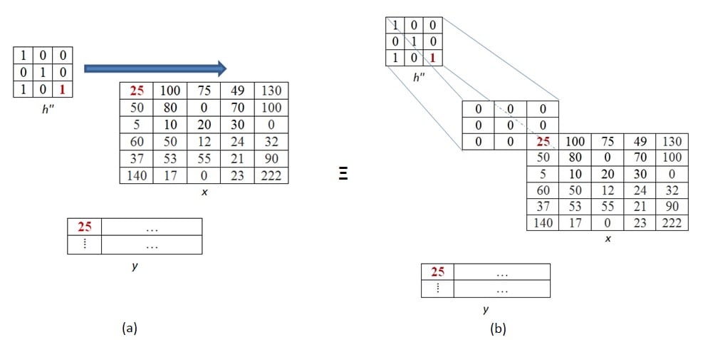
Figure 7: Zero-padding shown for the first pixel of the image (Drawn by me)

This process of adding extra zeros is known as zero padding and is required to be done in each case where there are no image pixels to overlap the kernel pixels. For our example, zero padding requires to be carried on for each and every pixel which lies along the first two rows and columns as well as those which appear along the last two rows and columns (these pixels are shown in blue font in Figure 8). In general, the number of rows or columns to be zero-padded on each side of the input image is given by (number of rows or columns in the kernel – 1).

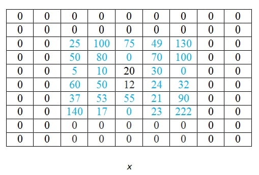
Figure 8

One important thing to be mentioned is the fact that zero padding is not the only way to deal with the edge effects brought about by convolution. Other padding techniques include replicate padding, periodic extension, mirroring, etc. (Digital Image Processing Using Matlab 2E, Gonzalez, Tata McGraw-Hill Education, 2009).

Summary

This article aims at explaining the graphical method of 2-D convolution and the concept of zero padding with respect to digital image processing.