Practical FIR Filter Design: Part 1

This tutorial will focus on designing a finite impulse response (FIR) filter. As the series progresses, it will discuss the necessary steps to implement the filter on real hardware.


A FIR filter is a digital filter whose impulse response settles to zero in finite time as opposed to an infinite impulse response filter (IIR), which uses feedback and may respond indefinitely to an input signal.The great thing about FIR filters is that they are inherently stable and can easily be designed to have linear phase. I won't get into the details much further on FIR filters and their pro's and con's as this tutorial focuses more on designing filters fast and efficiently with the aid of Octave.

Typically, in FIR filter design the length of the filter will need to be specified. You can guess and check until the filter matches your expected bandwidth and cutoff requirements, but this could be a long and tedious process. The equation below is an efficient way to compute a reasonable starting length. After trying the calculated N, one can then tweak N or parameters which make up N to meet filter specifications.

N≈AdBFs22Δf$$N\approx \frac{A_{dB}{F}_s}{22\mathrm{\Delta }f}$$

where

AdB$$A_{dB}$$

is your stopband attenuation in dB

Fs$$F_s$$

is your sampling frequency

and

Δf$$\mathrm{\Delta }f$$

is your transition bandwidth

Lets say we want to filter an audio signal with the following characteristics and desired filter response:
- The samples may contain frequencies from 0-20kHz
- We wish to design a filter that passes only frequencies less than 10kHz
- We want a stopband attenuation of 40 dB at 15kHz
- Our system has a

Fs$$F_s$$

of 192kHz

With this information we can begin the process of design. Using the equation for N we estimate the filter length to approximately be:

N≈(40)(192000Hz)22(15kHz−10kHz)$$N\approx \frac{(40)(192000Hz)}{22(15kHz-10kHz)}$$

N≈69.818$$N\approx 69.818$$

rounding to the nearest odd number

N≈69$$N\approx 69$$

*Designing an FIR filter length to be odd length will give the filter an integral delay of (N-1)/2.

Using the Octave/Matlab code below, we can see how to design a lowpass filter with a bandwidth of 10kHz and a cutoff of 15kHz using Octave's built in fir1 function, which is well documented here

                    close all;
clear all;
clf;


f1 = 10000;
f2 = 15000;
delta_f = f2-f1;
Fs = 192000;
dB  = 40;
N = dB*Fs/(22*delta_f);

f =  [f1 ]/(Fs/2)
hc = fir1(round(N)-1, f,'low')


figure
plot((-0.5:1/4096:0.5-1/4096)*Fs,20*log10(abs(fftshift(fft(hc,4096)))))
axis([0 20000 -60 20])
title('Filter Frequency Response')
grid on
                  

 

The code above gives us the following response:

Figure 1

But if we zoom in we will see that the attenuation at 10kHz is greater than 3dB: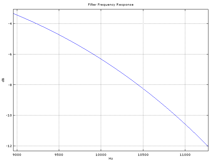

\

Figure 2

The bandwidth of the filter is always specified to the -3dB point, so in the first iteration of design our filter has a smaller bandwidth than specified (somewhere less than 9kHz). We can see from the first figure that the attenuation in the stopband exceeded our specifications, perhaps we can tweak the attenuation and passband frequency to enhance the design.

Tweaking the parameters in the code to

f1 = 11200;
f2 = 15000;
dB  = 30;

gives us a filter which closely matches our speicfications

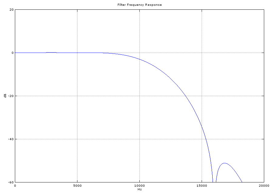
Figure 3

The filter design is now complete. Let's simulate how it works by adding the code below to the first bit of code we looked at.

                    x = sin(2*pi*[1:1000]*5000/Fs) +  sin(2*pi*[1:1000]*2000/Fs) + sin(2*pi*[1:1000]*13000/Fs)  + sin(2*pi*[1:1000]*18000/Fs);

sig = 20*log10(abs(fftshift(fft(x,4096))));
xf = filter(hc,1,x)

figure
subplot(211)
plot(x)
title('Sinusoid with frequency components 2000, 5000, 13000, and 18000 Hz')


subplot(212)
plot(xf)
title('Filtered Signal')
xlabel('time')
ylabel('amplitude')


x= (x/sum(x))/20
sig = 20*log10(abs(fftshift(fft(x,4096))));
xf = filter(hc,1,x)

figure
subplot(211)
plot((-0.5:1/4096:0.5-1/4096)*Fs,sig)
hold on
plot((-0.5:1/4096:0.5-1/4096)*Fs,20*log10(abs(fftshift(fft(hc,4096)))),'color','r')
hold off
axis([0 20000 -60 10])
title('Input to filter - 4 Sinusoids')
grid on
subplot(212)
plot((-0.5:1/4096:0.5-1/4096)*Fs,20*log10(abs(fftshift(fft(xf,4096)))))
axis([0 20000 -60 10])
title('Output from filter')
xlabel('Hz')
ylabel('dB')
grid on

                  

 

Figure 4

As we can see in Figure 4, we have the time domain signals on the left and the frequency domain on the right. The filter (in red) is overlaid onto the plot to show how the filter leaves the sinusoids in the passband and attenuates the signals in the transition and stopband.

The fir1 function can also be used to produce notch filters, high pass filters, and bandpass filters by replacing these lines:

f =  [f1 ]/(Fs/2), may need to be specified with two arguments for bandpass and notch filters as such:

f = [f1 f2]/(Fs/2), where f1 is the left -3dB edge and f2 is the right -3dB edge 

hc = fir1(round(N)-1, f,'low') can be modified as such:

'low' can be replaced with 'stop' (notch), 'high' (highpass), 'bandpass' (bandpass)

From the lowpass filter demonstration above it should be easy to form the coefficients (this is the variable hc in the code) for any filter desired. Once you have calculated the coefficients it is important to scale and quantize them so you can implement your filter in a microprocessor. In part 2 we will get into scaling the coefficients and other steps necessary to put your coefficients into an N-bit microprocessor. This is important because without proper scaling you will experience quanitization noise that will affect the frequency response of your filter. Consequently, your design will not match your original specification or the output you simulated in Octave.